Learning a parametrized intersection from a few training examples

Julia script for this example a) (joint image denoising+deblurring+inpainting)

Julia script for this example b) (image desaturation)

The applications of interest for this example are linear inverse problems, such as removing motion blur with a known blurring kernel and inpainting of missing pixels, single-image super-resolution, denoising, and desaturation of saturated images. We use aerial photos as the target. We can solve these various image processing tasks with the following simple strategy:

1. Observe the constraint parameters of various constraints in various transform-domains for all training examples (independently in parallel for each example and each constraint).
2. Add a data-fit constraint to the intersection.
3. The solution of the inverse problem is the projection of an initial guess \(m\) onto the learned intersection of sets \[ \begin{equation} \min_{x,\{y_i\}} \frac{1}{2}\| x - m \|_2^2 + \sum_{i=1}^{p-1} \iota_{\mathcal{C}_i}(y_i) + \iota_{\mathcal{C}_p^\text{data}}(y_p)\quad \text{s.t.} \quad \begin{cases} A_i x = y_i \\ Fx=y_p \end{cases}, \label{proj_intersect_lininvprob2} \end{equation} \] where \(F\) is a linear forward modeling operator and we solve this problem with

For both of the examples we observe the following constraint parameters from exemplar images:

1. \(\{ m \: | \: \sigma_1 \leq m[i] \leq \sigma_2 \}\) (upper and lower bounds)
2. \(\{ m \: | \: \sum_{j=1}^k \lambda[j] \leq \sigma_3 \}\) with \(m = \operatorname{vec}( \sum_{j=1}^{k}\lambda[j] u_j v_j^\top )\) is the SVD of the image (nuclear norm)
3. \(\{ m \: | \: \sum_{j=1}^k \lambda[j] \leq \sigma_4 \}\), with \((D_z \otimes I_x)m = \operatorname{vec}( \sum_{j=1}^{k}\lambda[j] u_j v_j^* )\) is the SVD of the vertical derivative of the image (nuclear norm of discrete gradients of the image, total-nuclear-variation). Use similar constraint for the x-direction.
4. \(\{ m \: | \: \| A m \|_1 \leq \sigma_5 \}\) with \(A = \begin{pmatrix} D_z \otimes I_x \\ I_z \otimes D_x \end{pmatrix}\) (anisotropic total-variation)
5. \(\{ m \: | \: \sigma_6 \leq \| m \|_2 \leq \sigma_7 \}\) (annulus)
6. \(\{ m \: | \: \sigma_8 \leq \| A m \|_2 \leq \sigma_9 \}\) with \(A = \begin{pmatrix} D_z \otimes I_x \\ I_z \otimes D_x \end{pmatrix}\) (annulus of the discrete gradients of the training images)
7. \(\{ m \: | \: \| A m \|_1 \leq \sigma_{10} \}\) with \(A = \) discrete Fourier transform (\(\ell_1\)-norm of DFT coefficients)
8. \(\{ m \: | \: - \sigma_{11} \leq ((D_z \otimes I_x) m)[i] \leq \sigma_{12} \}\) (slope-constraints in the \(z\)-direction, bounds on the discrete gradients of the image). Use similar constraint for the \(x\)-direction.
9. \(\{ m \: | \: \| A m \|_1 \leq \sigma_{11} \}\) with \(A = \) discrete wavelet transform

These are nine types of convex and non-convex constraints on the model properties (\(11\) sets passed to PARSDMM because sets three and eight are applied to the two dimensions separately). For data-fitting, we add a point-wise constraint, \(\{ x \: | \: l \leq (F x - d_\text{obs}) \leq u \}\) with a linear forward model \(F \in \mathbb{R}^{M \times N}\).

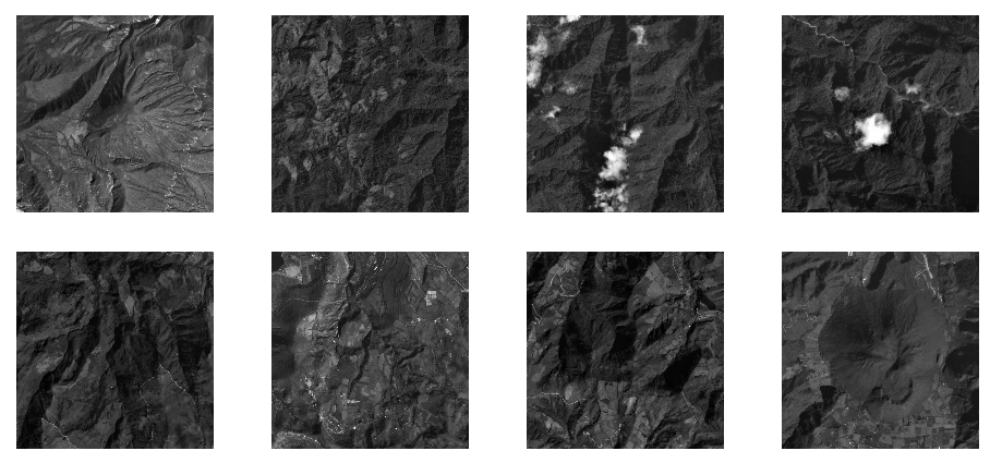
Example 1: joint denoising-deblurring-inpainting

The goal of the first example is to recover a \([0 - 255]\) grayscale image from \(20\%\) observed pixels of a blurred image (\(25\) pixels known motion blur), where each observed data point also contains zero-mean random noise in the interval \([-10 - 10]\). The forward operator \(F\) is thus a subsampled banded matrix (restriction of an averaging matrix). As an additional challenge, we do not assume exact knowledge of the noise level and work with the over-estimation \([-15 - 15]\). The data set contains a series of images from ‘Planet Labs PlanetScope Ecuador’ with a resolution of three meters, available at openaerialmap.org. There are \(35\) patches of \(1100 \times 1100\) pixels for training, some of which are displayed in Figure 1.

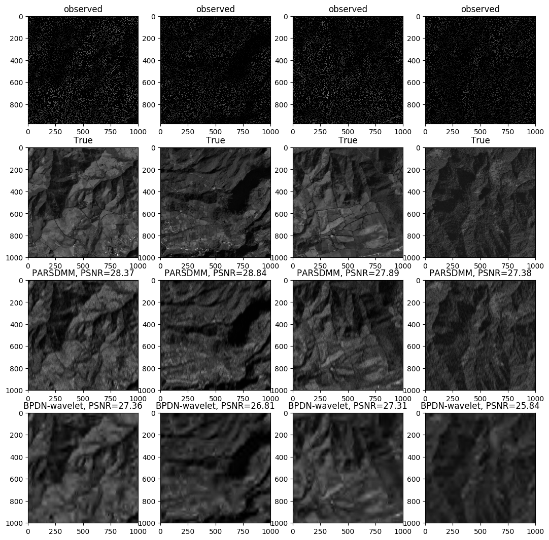
We compare the results of the proposed PARSDMM algorithm with the \(11\) learned constraints, with a basis pursuit denoise (BPDN) formulation. Basis-pursuit denoise recovers a vector of wavelet coefficients, \(c\), by solving \(\min_c \| c \|_1 \:\: \text{s.t.} \:\: \|F W^* c - d_\text{obs} \|_2 \leq \sigma\) (BPDN-wavelet) with the SPGL1 toolbox. The matrix \(W\) represents the wavelet transform: Daubechies Wavelets as implemented by the SPOT linear operator toolbox (http://www.cs.ubc.ca/labs/scl/spot/index.html) and computed with the Rice Wavelet Toolbox (RWT, github.com/ricedsp/rwt).

In Figure 2 we see that an overestimation of \(\sigma\) in the BPDN formulation results in oversimplified images, because the \(\ell_2\)-ball constraint is too large which leads to a coefficient vector \(c\) that has an \(\ell_1\)-norm that is smaller than the \(\ell_1\)-norm of the true image. The values for \(l\) and \(u\) in the data-fit constraint \(\{ x \: | \: l \leq (F x - d_\text{obs}) \leq u \}\), are also too large. However, the results from the projection onto the intersection of multiple constraints suffer much less from overestimated noise levels, because there are many other constraints that control the model properties. The results in Figure 2 show that the learned set-intersection approach achieves a higher PSNR for all evaluation images compared to the BPDN formulation.

Example 2: Image desaturation

To illustrate the versatility of the learning strategy, algorithm, and constraint sets from the previous example, we now solve an image desaturation problem for a different data set. The only two things that we change are the constraint set parameters, which we observe from new training images (Figure 3), and a different linear forward operator \(F\). The data set contains image patches (\(1500 \times 1250\) pixels) from the ‘Desa Sangaji Kota Ternate’ image with a resolution of \(11\) centimeters, available at openaerialmap.org. The corrupted observed images are saturated grayscale and generated by clipping the pixel values from \(0 - 60\) to \(60\) and from \(125 - 255\) to \(125\), so there is saturation on both the dark and bright pixels. If we have no other information about the pixels at the clipped value, the desaturation problem implies the point-wise bound constraints \[ \begin{equation} \begin{cases} 0 \leq x[i] \leq 60 & \text{if } d^{\text{obs}}[i] =60\\ x[i] = d^{\text{obs}}[i] & \text{if } 60 \leq d^{\text{obs}}[i] \leq 125\\ 125 \leq x[i] \leq 255 & \text{if } d^{\text{obs}}[i] = 125\\ \end{cases}. \label{saturation_constraint} \end{equation} \] The forward operator is thus the identity matrix. We solve problem \(\eqref{proj_intersect_lininvprob2}\) with these point-wise data-fit constraints and the model-property constraints listed in the previous example.

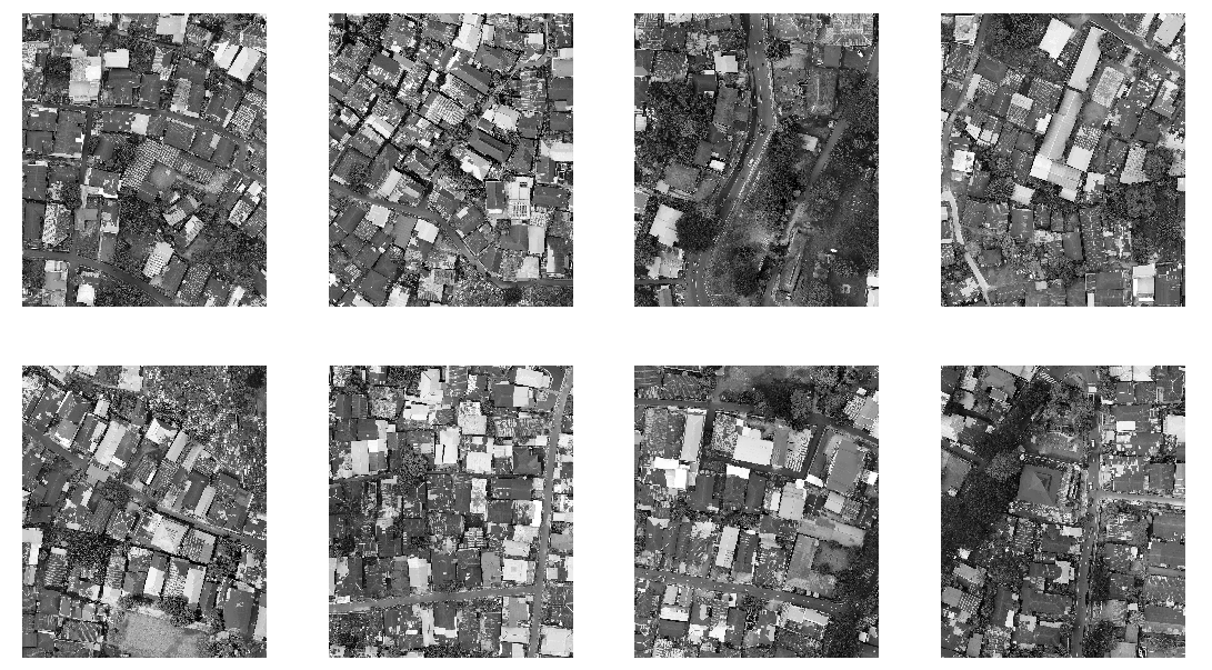
Figure 4 shows the results, true and observed data for four evaluation images. Large saturated patches are not desaturated accurately everywhere, because they contain no non-saturated observed pixels that serve as ‘anchor’ points.

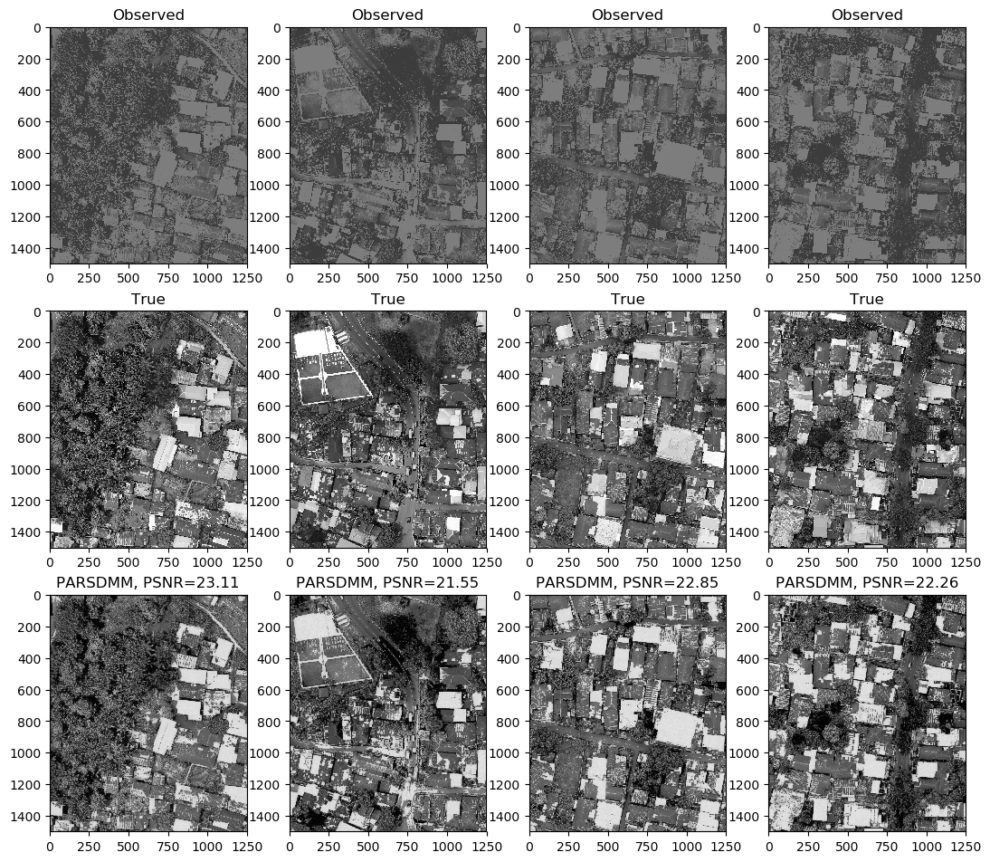
Both the desaturation and the joint deblurring-denoising-inpainting example show that PARSDMM with multiple convex and non-convex sets converges to good results, while only a few training examples were sufficient to estimate the constraint set parameters. Because of the problem formulation, algorithms, and simple learning strategy, there were no parameters to hand-pick.