Performance of Projection Adaptive Relaxed Simultaneous Method of Multipliers (PARSDMM)

Julia scripts for the examples on this page:
Parallel Dykstra’s algorithm vs PARSDMM
2D grid size vs time scaling
3D grid size vs time scaling

To see how the proposed PARSDMM algorithm compares to parallel Dykstra’s algorithm, we need to set up a fair experimental setting that includes the sub-problem solver in parallel Dykstra’s algorithm. Fortunately, if we use Adaptive Relaxed ADMM (ARADMM) for the projection sub-problems of parallel Dykstra’s algorithm, both PARSDMM and Parallel Dykstra-ARADMM have the same computational components. ARADMM also uses the same update scheme for the augmented Lagrangian penalty and relaxation parameters as we use in PARSDMM. This similarity allows for a comparison of the convergence as a function of the basic computational components. We manually tuned ARADMM stopping conditions to achieve the best performance for parallel Dykstra’s algorithm overall.

The numerical experiment is the projection of a 2D geological model (\(341 \times 400\) pixels) onto the intersection of three constraint sets that are of interest to seismic imaging:

1. \(\{ m \: | \: \sigma_1 \leq m[i] \leq \sigma_2 \}\) : bound constraints
2. \(\{ m \: | \: \| A m \|_1 \leq \sigma \}\) with \(A = [(I_x \otimes D_z)^\top \:\: (D_x \otimes I_z)^\top]^\top\) : anisotropic total-variation constraints
3. \(\{ m \: | \: 0 \leq ((I_x \otimes D_z) m)[i] \leq \infty \}\) : vertical monotonicity constraints

For these sets, the primary computational components are (i) matrix-vector products in the conjugate-gradient algorithm. The system matrix has the same sparsity pattern as \(A^\top A\), because the sparsity patterns of the linear operators in set number one and three overlap with the pattern of \(A^\top A\). Parallel Dykstra uses matrix-vector products with \(A^\top A\), \((D_x \otimes I_z)^\top (D_x \otimes I_z)\), and \(I\) in parallel. (ii) projections onto the box constraint set and the \(\ell_1\)-ball. Both parallel Dykstra’s algorithm and PARSDMM compute these in parallel. (iii) parallel communication that sends a vector from one to all parallel processes, and one map-reduce parallel sum that gathers the sum of vectors on all workers. The communication is the same for PARSDMM and parallel Dykstra’s algorithm so we ignore it in the experiments below.

Before we discuss the numerical results, we discuss some details on how we count the computational operations mentioned above:

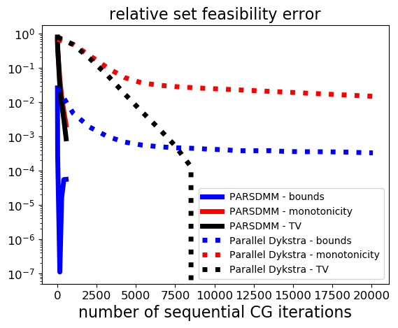
• Matrix-vector products in CG: At each PARSDMM iteration, we solve a single linear system with the conjugate-gradient method. Parallel Dykstra’s algorithm simultaneously computes three projections by running three instances of ARADMM in parallel. The projections onto sets two and three solve a linear system at every ARADMM iteration. For each parallel Dykstra iteration, we count the total number of sequential CG iterations, which is determined by the maximum number of CG iterations for either set number two or three.

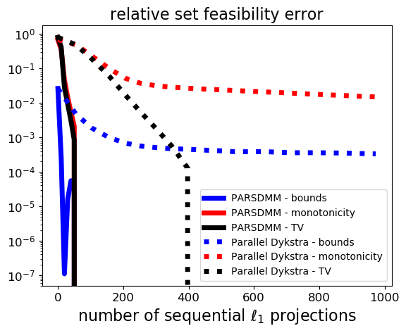
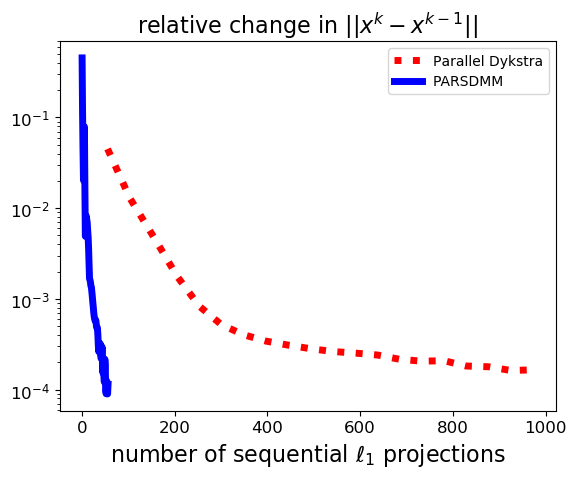
• \(\ell_1\)-ball projections: PARSDMM projects onto the \(\ell_1\) ball once per iteration. Parallel Dykstra projects (number of parallel Dykstra iterations) \(\times\) (number of ARADMM iterations for set number two) times onto the \(\ell_1\) ball. Because \(\ell_1\)-ball projections are computationally more intensive compared to projections onto the box (element-wise comparison) and also less suitable for multi-threaded parallelization, we focus on the \(\ell_1\)-ball projections.

We use the following stopping criteria: \[ \begin{equation} r^\text{evol} < \varepsilon^\text{evol} \quad \text{and} \quad r^{\text{feas}}_i < \varepsilon^{\text{feas}}_i \quad \forall \: i. \label{stopping_conditions} \end{equation} \] with \[ \begin{equation} r^{\text{feas}}_i = \frac{ \| A_i x - \mathcal{P}_{\mathcal{C}_i}(A_i x) \| }{ \| A_i x \| }, \, i=1\cdots p, \label{feas_stop} \end{equation} \] and \[ \begin{equation} r^\text{evol} = \frac{ \text{max}_{j \in S} \{ \|x^k - x^{k-j}\| \} }{ \|x^k\| }, \label{obj_stop} \end{equation} \] where \(S \equiv \{ 1,2,\dots,5 \}\). During our numerical experiments, we select \(\varepsilon^\text{evol}=10^{-2}\) and \(\varepsilon^{\text{feas}}_i = 10^{-3}\), which balance sufficiently accurate solutions and short solution times.

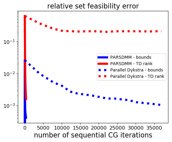
The results in Figure 1 show that PARSDMM requires much fewer CG iterations and \(\ell_1\)-ball projections to achieve the same relative set feasibility error in the transform-domain as defined in equation \(\eqref{feas_stop}\). Different from the curves corresponding to parallel Dykstra’s algorithm, we see that PARSDMM converges somewhat oscillatory, which is caused by changing the relaxation and augmented-Lagrangian penalty parameters.

Because non-convex sets are an important application for us, we compare the performance for a non-convex intersection as well:

1. \(\{ m \: | \: \sigma_1 \leq m[i] \leq \sigma_2 \}\): bound constraints
2. \(\{ m \: | \: (I_x \otimes D_z) m = \operatorname{vec}( \sum_{j=1}^{r}\lambda[j] u_j v_j^* )\}\), where \(r < \text{min}(n_z,n_x)\), \(\lambda[j]\) are the singular values, and \(u_j\), \(v_j\) are singular vectors: rank constraints on the vertical gradient of the image

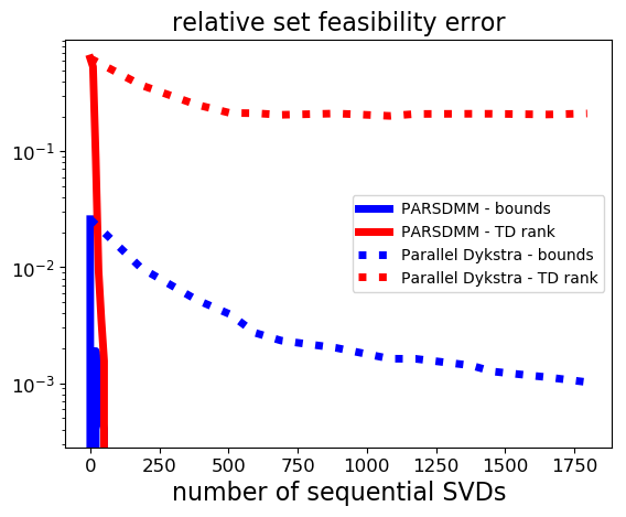
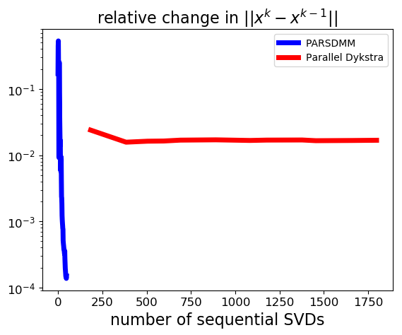
We count the computational operations in the same way as in the previous example, but this time the computationally most costly projection is the projection onto the set of matrices with limited rank via the singular value decomposition. The results in Figure 2 show that the convergence of parallel Dykstra’s algorithm almost stalls: the solution estimate gets closer to satisfying the bound constraints, but there is hardly any progress towards the rank constraint set. PARSDMM does not seem to suffer from non-convexity in this particular example.

We used the single-level version of PARSDMM such that we can compare the computational cost with Parallel Dykstra. The PARSDMM results in this section are therefore pessimistic in general, as the multilevel version can offer additional speedups, which we show next.

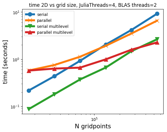
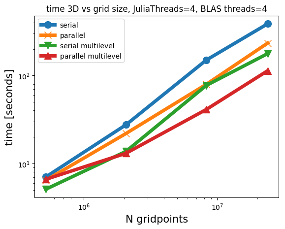
Some timings for 2D and 3D projections

We show timings for projections of geological models onto two different intersections for the four modes of operation: PARSDMM, parallel PARSDMM, multilevel PARSDMM, and multilevel parallel PARSDMM. As we mentioned, the multilevel version has a small additional overhead compared to single-level PARSDMM because of one interpolation procedure per level. Parallel PARSDMM has communication overhead compared to serial PARSDMM. However, serial PARSDMM still uses multi-threading for projections, the matrix-vector product in the conjugate-gradient method, and BLAS operations, but the \(y_i\) and \(v_i\) computations in Algorithm #alg:PARSDMM remain sequential for every \(i=1,2,\cdots,p, p+1\), contrary to parallel PARSDMM. We carry our computations out on a dedicated cluster node with \(2\) CPUs per node with 10 cores per CPU (Intel Ivy Bridge 2.8 GHz E5-2680v2) and 128 GB of memory per node.

The following sets have been used to regularize geophysical inverse problems and form the intersection for our first test case:

1. \(\{ m \: | \: \sigma_1 \leq m[i] \leq \sigma_2 \}\) : bound constraints
2. \(\{ m \: | \: -\sigma_3 \leq ((D_x \otimes I_z) m)[i] \leq \sigma_3 \}\): lateral smoothness constraints. There are two of these constraints in the 3D case: for the \(x\) and \(y\) direction separately.
3. \(\{ m \: | \: 0 \leq ((I_x \otimes D_z) m)[i] \leq \infty \}\) : vertical monotonicity constraints

The results in Figure 3 show that the multilevel strategy is much faster than the single-level version of PARSDMM. The multilevel overhead costs are thus small compared to the speedup. It also shows that, as expected, the parallel versions require some communication time, so the problems need to be large enough for the parallel version of PARSDMM to offer speedups compared to its serial counterpart.